R “driving” PostGIS
tstartpg <- Sys.time()
if (!require("pacman")) install.packages("pacman")
pacman::p_load(
    tidycensus,
    htmltools,
    sf,
    tidyverse,
    magrittr,
    geojsonsf,
    ggplot2
)

# this loads the proper $PATH on our Windows Server for OSGEO
path <- "C:\\PROGRA~1\\QGIS32~1.0\\apps\\qt5\\bin;C:\\PROGRA~1\\QGIS32~1.0\\apps\\Python39\\Scripts;C:\\PROGRA~1\\QGIS32~1.0\\bin;C:\\WINDOWS\\system32;C:\\WINDOWS;C:\\WINDOWS\\system32\\WBem"
Sys.setenv(PATH = path)

# convert wkb if necessary
f_ewkb_to_sf <- function(x, spatial_column) {
    cmd <- paste("x %<>% mutate(geometry = st_as_sfc(structure(as.list(", spatial_column, "), class = 'WKB'), EWKB = TRUE))")
    eval(parse(text = cmd))
    x <- st_as_sf(x, sf_column_name = "geometry")
    cmd <- paste("x %<>% dplyr::select(-", spatial_column, ")")
    eval(parse(text = cmd))
    x
}

knitr::opts_chunk$set(echo = TRUE, warning = FALSE, message = FALSE)
1 Introduction
For this section, we will perform the same analysis as we did using sf, but this time using PostGIS for the analytic functions. The framework is still in R, with database functions performed using commands from the DBI package, e.g., dbGetQuery() for generic SQL commands and dbWriteTable() for writing sf data frames to the database. Additionally, the GDAL/OGR tools are used for writing spatial formats directly to the database.
2 Bring data into PostGIS
The code chunk below loads some functions for connecting to a PostgreSQL database, and then connects to a database that has the PostGIS extension installed.
source("dbconnect.R")
pmh <- phurvitz <- connectdb(host = "doyenne", dbname = "phurvitz", user = Sys.getenv("pguser"), password = Sys.getenv("pgpassword"))
2.1 Block group data
The code below downloads the block group data using tidycensus for and then writes to a PostGIS database.
# get the data
bg <- get_acs(
    geography = "block group",
    variables = c(
        pop_total = "B01003_001",
        pop_white = "B02001_002",
        pop_income_below_pov = "B17010_002",
        pop_ed_lt_hs = "B28006_003"
    ),
    year = 2020,
    state = "WA",
    county = "King",
    geometry = TRUE,
    output = "wide",
    progress_bar = FALSE
) %>%
    st_transform(26910) %>%
    select(everything(), geom_26910 = geometry) %>%
    select(-NAME)

names(bg) %<>% str_to_lower() %>% str_replace_all(pattern = "e$", replacement = "")

# create a schema
O <- dbGetQuery(conn = pmh, statement = "create schema if not exists cugos_2023;")
# a temporary schema
O <- dbGetQuery(conn = pmh, statement = "create schema if not exists tmp;")

# write BG to the database
# I'm having trouble with PostgreSQL drivers, so write out and then alter the column
st_write(obj = bg, dsn = "PG:host=doyenne dbname=phurvitz", layer = "bg", layer_options = c("schema=cugos_2023", "geometry_name=geom_26910", "overwrite=yes"), quiet = TRUE)
Let’s take a quick look at the block groups (Figure 2.1), as ugly as it is floating in coordinate space without neighboring geographies!.
# pull from db
bg_pg <- st_read(dsn = "PG:host=doyenne dbname=phurvitz", layer = "cugos_2023.bg", quiet = TRUE) %>%
    mutate(pct_nonwhite = ((pop_total - pop_white) / pop_total * 100) %>% round(1))

# as sf
bg_pg %>% ggplot() +
    geom_sf()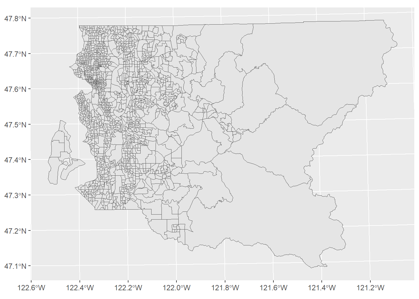
Figure 2.1: Block groups
Here we can see a histogram of the data (Figure 2.2), the count of block groups by percent non-white.
bg_pg %>%
    arrange(pct_nonwhite) %>%
    ggplot(mapping = aes(x = pct_nonwhite)) +
    geom_histogram(bins = 100) +
    xlab("% nonwhite") +
    ylab("count of block groups")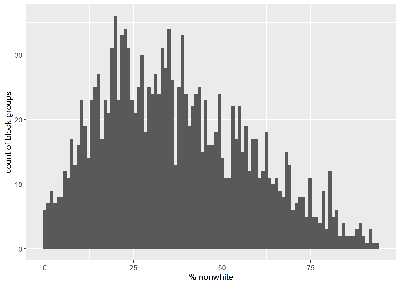
Figure 2.2: Percent nonwhite
2.2 Water area data
The water area data can be downloaded as a zipped shape file. ogr2ogr includes GDAL Virtual File Systems, allowing streaming input to the database from compressed formats and even URLs. Here we prepend /vsizip/vsicurl to the data source in order for it to be read in this way.
For shape files, the layer name matches the shape file name, so under the assumption that the TIGER/Line .zip files are named rationally, we can predict the layer name.
# this pushes the water data to the db
cmd <- 'cmd /c ogr2ogr -f PostgreSQL PG:"host=doyenne, dbname=phurvitz"
"/vsizip/vsicurl/https://www2.census.gov/geo/tiger/TIGER2021/AREAWATER/tl_2021_53033_areawater.zip"
tl_2021_53033_areawater
-nln water
-lco overwrite=yes
-lco schema=cugos_2023
-a_srs EPSG:4326 -t_srs EPSG:26910
-lco geometry_name=geom_26910' %>% str_replace_all(pattern = "\n", " ")
O <- system(cmd)
The water areas are shown in Figure 2.3.
# pull from db
w <- st_read(dsn = "PG:host=doyenne dbname=phurvitz", layer = "cugos_2023.water", quiet = TRUE)

w %>% ggplot() +
    geom_sf(fill = "cyan", color = "cyan")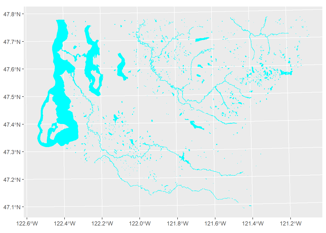
Figure 2.3: King County water areas from US Census TIGER/Line data
Water areas are erased in the large SQL query for the overlay analysis, below.
2.3 Seattle Neighborhoods
We will use the OSGEO utilities ogrinfo to get information about the Seattle neighborhoods data set, since for GeoJSON files, the layer name within the data source does not necessarily match the data source name. Also in this case the URL is quite arcane (we obtained the URL from interactively using the Seattle GeoData web site.
cmd <- 'cmd /c ogrinfo
"https://opendata.arcgis.com/api/v3/datasets/b4a142f592e94d39a3bf787f3c112c1d_0/downloads/data?format=geojson&spatialRefId=4326&where=1%3D1"' %>%
    str_replace_all(pattern = "\n", replacement = "")
system(cmd, intern = TRUE)
## [1] "INFO: Open of `https://opendata.arcgis.com/api/v3/datasets/b4a142f592e94d39a3bf787f3c112c1d_0/downloads/data?format=geojson&spatialRefId=4326&where=1%3D1'"
## [2] " using driver `GeoJSON' successful."
## [3] "1: Neighborhood_Map_Atlas_Neighborhoods"Next we will use ogr2ogr to import the Seattle neighborhoods directly from the GeoJSON URL into the PostGIS database, also transforming the coordinates from EPSG 4326 (Geographic WGS84) to EPSG 26910 (UTM 10 N NAD83) during the import. Note that the layer name within the ogr2ogr command was obtained above using ogrinfo.
# this pushes the neighborhoods data
cmd <- 'cmd /c ogr2ogr -f PostgreSQL PG:"host=doyenne, dbname=phurvitz"
"https://opendata.arcgis.com/api/v3/datasets/b4a142f592e94d39a3bf787f3c112c1d_0/downloads/data?format=geojson&spatialRefId=4326&where=1%3D1"
Neighborhood_Map_Atlas_Neighborhoods
-nln nhood
-lco overwrite=yes
-lco schema=cugos_2023
-a_srs EPSG:4326 -t_srs EPSG:26910
-lco geometry_name=geom_26910' %>% str_replace_all(pattern = "\n", " ")
O <- system(cmd)

nh <- st_read(dsn = "PG:host=doyenne dbname=phurvitz", layer = "cugos_2023.nhood", quiet = TRUE)

nh %>% ggplot() +
    geom_sf()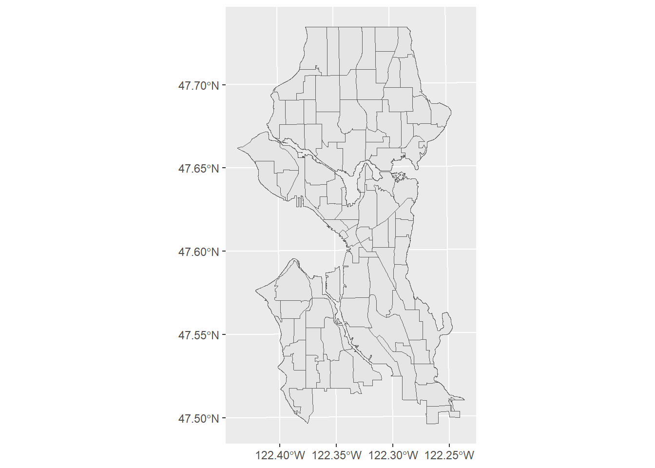
We demonstrate that the data align (Figure 2.4).
ggplot() +
    geom_sf(data = bg_pg) +
    geom_sf(data = nh, color = "cyan", fill = NA)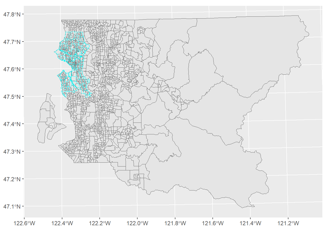
Figure 2.4: King County block groups and Seattle neighborhoods
3 Overlay analysis within PostGIS
To take advantage of the speed of using spatial indexes, we will create tables for each intermediate output and create indexes on those.
t0 <- Sys.time()

# BG slivers
sql_select_bg <- "
--union the neighborhood geoms
drop table if exists tmp.nhood;
create table tmp.nhood as
select st_union(geom_26910) as geom_26910 from cugos_2023.nhood;
create index if not exists idx_tmp_nhood on tmp.nhood using gist (geom_26910);

-- select BGs within the city
drop table if exists tmp.bg_nhood;
create table tmp.bg_nhood as
select b.*
from cugos_2023.bg as b
   , tmp.nhood as n
where st_intersects(b.geom_26910, n.geom_26910);
create index idx_tmp_bg_nhood on tmp.bg_nhood using gist (geom_26910);

-- a single water polygon
drop table if exists tmp.wateru;
create table tmp.wateru as
select 1, st_union(geom_26910) as geom_26910
from cugos_2023.water;
create index idx_tmp_wateru on tmp.wateru using gist (geom_26910);

-- clip by water
drop table if exists tmp.bg_water;
create table tmp.bg_water as
with a as
    -- clip those that overlap with water
    (select true                                      as clip
          , b.geoid
          , b.pop_total
          , b.pop_totalm
          , b.pop_white
          , b.pop_whitem
          , b.pop_income_below_pov
          , b.pop_income_below_povm
          , b.pop_ed_lt_hs
          , b.pop_ed_lt_hsm
          , st_difference(b.geom_26910, w.geom_26910) as geom_26910
     from tmp.bg_nhood as b
        , tmp.wateru as w
     where st_intersects(b.geom_26910, w.geom_26910))
   -- those that did not overlap with water
   , x as (select false as clip
                , b.geoid
                , b.pop_total
                , b.pop_totalm
                , b.pop_white
                , b.pop_whitem
                , b.pop_income_below_pov
                , b.pop_income_below_povm
                , b.pop_ed_lt_hs
                , b.pop_ed_lt_hsm
                , b.geom_26910
           from tmp.bg_nhood as b
           where geoid not in (select geoid from a))
-- union
   , u as (
    select *
    from a
    union all
    select *
    from x)
--include area
select *, st_area(geom_26910) as area_m_bg_orig
from u;
create index idx_tmp_bg_water on tmp.bg_water using gist (geom_26910);

-- intersect with neighborhoods
drop table if exists cugos_2023.bg_nhood;
create table cugos_2023.bg_nhood as
with
-- intersection
    i0  as (select n.s_hood
                 , b.pop_total
                 , b.pop_white
                 , b.pop_total - b.pop_white                                                                     as pop_nonwhite
                 , b.pop_income_below_pov
                 , b.pop_ed_lt_hs
                 , b.area_m_bg_orig
                 , st_area(st_multi(st_intersection(b.geom_26910, n.geom_26910))::geometry(multipolygon, 26910)) as area_m_bg_clip
                 , st_multi(st_intersection(b.geom_26910, n.geom_26910))::geometry(multipolygon, 26910)          as geom_26910
            from tmp.bg_water as b
               , cugos_2023.nhood as n
            where st_intersects(b.geom_26910, n.geom_26910)
              and n.s_hood <> '000')
-- calculate area weighted estimates
   , c0 as
    (select *
          , area_m_bg_clip
            /
            area_m_bg_orig as
            area_prop
     from i0)
   , c1 as
    (select s_hood
          , pop_total * area_prop            as pop_total
          , pop_white * area_prop            as pop_white
          , pop_nonwhite * area_prop         as pop_nonwhite
          , pop_income_below_pov * area_prop as pop_income_below_pov
          , pop_ed_lt_hs * area_prop         as pop_ed_lt_hs
          , geom_26910
     from c0)
   -- aggregate by s_hood
   , a  as
    (select s_hood
          , sum(pop_total)                                                as pop_total
          , sum(pop_white)                                                as pop_white
          , sum(pop_nonwhite)                                             as pop_nonwhite
          , sum(pop_income_below_pov)                                     as pop_income_below_pov
          , sum(pop_ed_lt_hs)                                             as pop_ed_lt_hs
          , st_multi(st_union(geom_26910))::geometry(multipolygon, 26910) as geom_26910
     from c1
     group by s_hood)
   , c2 as
    (select *
          , round((pop_white / pop_total * 100)::numeric, 2)            as pct_white
          , round((pop_nonwhite / pop_total * 100)::numeric, 2)         as pct_nonwhite
          , round((pop_income_below_pov / pop_total * 100)::numeric, 2) as pct_income_below_pov
          , round((pop_ed_lt_hs / pop_total * 100)::numeric, 2)         as pct_ed_lt_hs
     from a)
select *
from c2;
"

O <- dbGetQuery(conn = pmh, statement = sql_select_bg)
atime <- difftime(Sys.time(), t0, units = "secs") %>%
    as.numeric() %>%
    round(2)
[The overlay analysis using PostGIS methods took 3.9 seconds.]
Figure 3.1 shows a simple map with the area-weighted estimate of the percent of residents below poverty.
# get the data
bg_nhood <- st_read(dsn = "PG:host=doyenne dbname=phurvitz", layer = "cugos_2023.bg_nhood", quiet = TRUE)

bg_nhood %>% ggplot() +
    geom_sf(aes(fill = pct_income_below_pov)) +
    labs(fill = "% below\npoverty")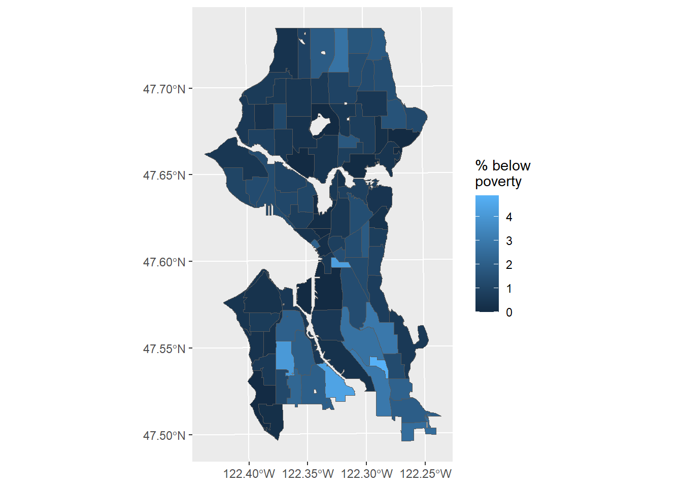
Figure 3.1: Estimate of percent below poverty in Seattle neighborhoods
pgrendertime <- difftime(Sys.time(), tstartpg, units = "secs") %>%
    as.numeric() %>%
    round(2)
Total render time with PostGIS: 34.87 seconds.
The total rendering time for all processes within R was 38.74 seconds, whereas with PostGIS it was 34.87 seconds. One of the operational differences, however, is that the PostGIS data are now stored in a database that can be used later without re-downloading, and the data are usable within a SQL framework without loading as R data frames.