Analytic outputs
tstartpg <- Sys.time()
library(tidycensus)
library(htmltools)
library(sf)
library(tidyverse)
library(magrittr)
library(leaflet)
library(ggplot2)
library(plotly)
library(viridis)
library(dichromat)

source("dbconnect.R")
pmh <- phurvitz <- connectdb(host = "doyenne", dbname = "phurvitz")

# convert wkb
f_ewkb_to_sf <- function(x, spatial_column) {
    cmd <- paste("x %<>% mutate(geometry = st_as_sfc(structure(as.list(", spatial_column, "), class = 'WKB'), EWKB = TRUE))")
    eval(parse(text = cmd))
    x <- st_as_sf(x, sf_column_name = "geometry")
    cmd <- paste("x %<>% dplyr::select(-", spatial_column, ")")
    eval(parse(text = cmd))
    x
}

knitr::opts_chunk$set(echo = TRUE, warning = FALSE, message = FALSE)
Here we present a few output objects.
1 Demographics by neighborhood
The two input data sets were census block groups and neighborhoods. The reason for the analysis is that the census data are not indexed to neighborhood and the neighborhood data do not contain demographic information. For this reason, GIS analysis is needed to conflate the data. Combining the data may lead to new insights about the demographic conditions in Seattle neighborhoods for the purpose of interventions or policy.
1.1 Race and poverty
bg_nhood_pg <- dbGetQuery(conn = pmh, statement = "select * from cugos_2023.bg_nhood;")

bg_nhood_pg <- f_ewkb_to_sf(x = bg_nhood_pg, spatial_column = "geom_26910")

# correlation
cor_est <- cor.test(bg_nhood_pg$pct_nonwhite, bg_nhood_pg$pct_income_below_pov)$estimate %>% round(2)
Figure 1.1 presents a scatter plot comparing estimates of percent nonwhite and percent living below federal poverty. level in 2021. The correlation coefficient was 0.66. Hover over points to see the values of % nonwhite, % below poverty level, and neighborhood name. The magnitude of persons living below the federal poverty level is relatively low.
p <- bg_nhood_pg %>% ggplot(mapping = aes(x = pct_nonwhite, y = pct_income_below_pov, text = s_hood)) +
    geom_point() +
    # geom_smooth() +
    xlab("% nonwhite") +
    ylab("% below poverty level")

ggplotly(p)
Figure 1.1: Percent nonwhite and income below poverty level estimated for Seattle neighborhoods, 2021
1.2 Education and poverty
A graph showing the relationship between poverty and education, including a locally smoothed trend line with confidence intervals is shown in 1.2. Although the trend is similar in shape and direction, there are relatively few persons over age 25 in the Seattle area with less than a high school education, compared to the number of nonwhite persons.
bg_nhood_pg %>% ggplot(mapping = aes(x = pct_ed_lt_hs, y = pct_income_below_pov)) +
    geom_point() +
    geom_smooth() +
    xlab("% with less than a high school education") +
    ylab("% below poverty level")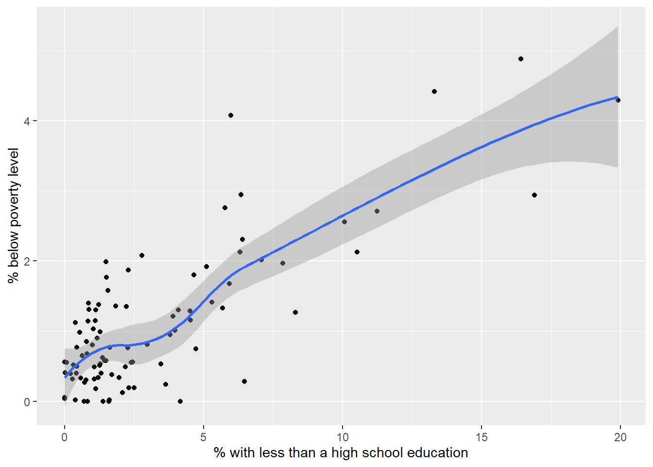
Figure 1.2: Percent nonwhite and income below poverty level estimated for Seattle neighborhoods with trend line, 2021
1.3 Race and education
The last graph (1.3 compares race and education. Here we see the same pattern; neighborhoods with greater proportion of nonwhite residents also have a higher proportion of persons wit less than a high school education.
bg_nhood_pg %>% ggplot(mapping = aes(x = pct_nonwhite, y = pct_ed_lt_hs)) +
    geom_point() +
    geom_smooth() +
    xlab("% nonwhite") +
    ylab("% with less than a high school education")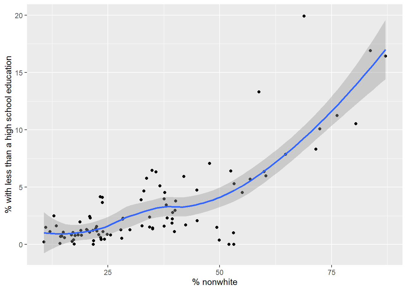
Figure 1.3: Percent nonwhite and percent with less than a high school education estimated for Seattle neighborhoods with trend line, 2021
2 Map interface
The final output is a Leaflet map.
Hover over a polygon to display a label of the neighborhood name. Zoom with mouse wheel, pan with middle or left button.
# project for map
bg_nhood_pg_4326 <- bg_nhood_pg %>% st_transform(4326)

# color palettes
pal_nonwhite <- colorNumeric(palette = "viridis", domain = bg_nhood_pg_4326$pct_nonwhite, n = 5)
pal_poverty <- colorNumeric(palette = "inferno", domain = bg_nhood_pg_4326$pct_income_below_pov, n = 5)
pal_edu <- colorNumeric(palette = topo.colors(5), domain = bg_nhood_pg_4326$pct_ed_lt_hs, n = 5)

# group names
nnw <- "% nonwhite"
nbp <- "% below poverty"
nle <- "% < HS"

# labels
labels_nonwhite <- paste0(bg_nhood_pg_4326$s_hood, "<br>nonwhite: ", bg_nhood_pg_4326$pct_nonwhite, "%") %>%
  lapply(htmltools::HTML)
labels_poverty <- paste0(bg_nhood_pg_4326$s_hood, "<br>below poverty: ", bg_nhood_pg_4326$pct_income_below_pov, "%") %>%
  lapply(htmltools::HTML)
labels_edu <- paste0(bg_nhood_pg_4326$s_hood, "<br>< HS: ", bg_nhood_pg_4326$pct_ed_lt_hs, "%") %>%
  lapply(htmltools::HTML)

m <- leaflet(data = bg_nhood_pg_4326, height = 1000) %>%
    # Base groups
    addTiles(group = "OSM (default)") %>%
    addProviderTiles(providers$Stamen.Toner, group = "Toner") %>%
    addProviderTiles(providers$Stamen.TonerLite, group = "Toner Lite") %>%
    # overlay groups (polygons)
    addPolygons(
        label = ~labels_nonwhite,
        weight = 2,
        fillColor = ~ pal_nonwhite(pct_nonwhite),
        fillOpacity = 0.8,
        group = nnw,
        labelOptions = labelOptions(textsize = "12px")
    ) %>%
    addPolygons(
        label = ~labels_poverty,
        weight = 2,
        fillColor = ~ pal_poverty(pct_income_below_pov),
        fillOpacity = 0.8,
        group = nbp,
        labelOptions = labelOptions(textsize = "12px")
    ) %>%
    addPolygons(
        label = ~labels_edu,
        weight = 2,
        fillColor = ~ pal_edu(pct_ed_lt_hs),
        fillOpacity = 0.8,
        group = nle,
        labelOptions = labelOptions(textsize = "12px")
    ) %>%
    # legends
    addLegend("bottomright",
        pal = pal_nonwhite, title = nnw,
        values = bg_nhood_pg_4326$pct_nonwhite, group = nnw
    ) %>%
    addLegend("bottomright",
        pal = pal_poverty, title = nbp,
        values = bg_nhood_pg_4326$pct_income_below_pov, group = nbp
    ) %>%
    addLegend("bottomright",
        pal = pal_edu, title = nle,
        values = bg_nhood_pg_4326$pct_ed_lt_hs, group = nle
    ) %>%
    # Layers control
    addLayersControl(
        baseGroups = c("OSM (default)", "Toner", "Toner Lite"),
        overlayGroups = c(nnw, nbp, nle),
        options = layersControlOptions(collapsed = FALSE)
    ) %>%
    # hide overlay groups to start
    hideGroup(c(nnw, nbp, nle))

m