Overview:
Vector
Raster
Displaying Vector & Raster Data
There are 2 basic data structures in GIS:
These features are the basic features in a vector-based GIS, such as ARC/INFO.
Points represent discrete locations on the ground. Either these are true points, such as survey markers, or they may be virtual points, based on the scale of representation. For example, a city's location on a driving map of the United States is represented by a point, even though in reality a city has area.
Points are accompanied by a point attribute table (PAT), which contains a record for each point. The records hold attributes for the point, such as city name, sampling point number, or radio tower frequency. More on attribute tables later in Week 2.
Lines represent linear features, such as rivers, roads and transmission cables.
In ARC/INFO, lines are known as "arcs," hence the name "ARC/INFO" (the "INFO" refers to the relational database INFO).
Arcs are composed of nodes and vertices. Arcs begin and end at nodes, and may have 0 or more vertices between the nodes. Arcs which connect share a common node.
The arc-node topology data model is central to ARC/INFO vector operations. Arcs are represented with starting and ending nodes, which imparts directionality to the arcs. They also are marked with left- and right-polygons.
Polygons are the most complex of vector data sets. They are composed of bounding arcs and label points. The bounding arcs are what keep track of the location of each polygon (each arc knows which polygon is on its left and right sides). The label points are markers which store attribute information for the entire polygon.
Tics manage the georeferencing of all vector data sets in ARC/INFO. The tics are registered to ground coordinates, and all other data in the coverage are in referenced to the tics (which in turn makes the features referenced to ground coordinates).
Here we have an example of a polygon coverage, displaying its arcs, label points, and tics. As you can see, polygon 3 is bounded by arcs 1, 3, and 4.
Arc 4 starts at node 3 and goes to node 2. Its right-hand polygon is 3, and its left-hand polygon is 1 (known as the universe polygon).
ARC/INFO automatically stores line length and polygon area in the units of measure defined by the user. These units can be feet, meters, or whatever units the user needs. The topic of units will be covered in more detail in the section on map projection.
In ARC/INFO there are 2 major implementations of vector data:
Coverages are a basic implementation of the vector arc-node topological model as described above.
Shape Files are a recent addition to the vector model, used mainly in ArcView. Although shape files do contain points, lines, and polygons, a single shape file can contain only one of these features. Coverages, on the other hand, can be composed of points, lines, polygons, points+lines, or lines+polygons. Shape files will be discussed during the unit on data conversion.
While polygons are composed of arcs and label points, and adjacent polygons share common arcs, adjacent shape polygons are completely separate objects. And while connecting arcs share common nodes, "connecting" shape lines do not really connect at all.
Moss Files are used in the public-domain GIS MOSS (Map Overlay and Statistical System), and are also used as input to the UCELL5 program in LMS. MOSS files are generated from coverages using the ARCMOSS command in ARC. MOSS files are simple ASCII files, listing feature numbers, a feature attribute, and the feature's and coordinates. Here are a few examples:
    1                1
 1551491.25  851667.06
    2                1
 1551490.00  851615.63
    3                1
 1551488.75  851561.31
    4                1
 1551487.63  851508.44
    5                1
 1551855.38  851476.19
    6                1
 1551268.25  851463.13
    7                1
 1551486.25  851454.06
    8                1
 1551198.25  851450.88
    9                1
 1551292.38  851448.69
   10                1
 1551352.50  851447.31
   11                1
 1551382.63  851446.63
|
1 EAST 2ND 2 543702.63 638368.25 543409.13 638369.00 2 EAST 2ND 2 547752.25 638261.63 548558.63 638266.13 3 EAST 3RD 11 543768.00 638025.88 543825.50 638037.88 543906.00 638045.00 543970.50 638047.63 543970.50 638047.63 544000.50 638046.13 544028.00 638040.25 544055.50 638029.25 544080.00 638014.38 544092.50 637999.38 544200.63 637900.00 4 EAST 3RD 2 548560.38 638006.75 547750.25 638010.13 5 EAST 3RD 2 548813.75 638046.25 548994.00 638046.00 6 EAST 3RD 2 548994.00 638046.00 549069.00 638046.00 |
       2          PF    681
 1199583.25  548529.00
 1199583.13  548522.44
 1199563.63  548076.50
...
 1197151.13  557021.56
 1197170.00  557592.25
 1197179.00  557843.13
    3          OTH      6
 1197179.00  557843.13
 1197170.00  557592.25
 1197151.13  557021.56
 1196582.75  557039.56
 1196608.38  557864.56
 1197179.00  557843.13
    4          OTH     15
 1198365.88  552553.69
 1200992.13  552460.44
...
|
Points are single records, listing the point number, optional attributes, number of coordinates (always 1 for points), and coordinates.
Lines are multi-coordinate records, listing the line number, optional attributes, number of coordinates, and coordinates for each node and vertex.
Polygons are also multi-coordinate records, listing the polygon number, optional attributes, number of coordinates, and coordinates for each node and vertex on the bounding arc. Polygons are stored differently than arcs, in that they always form closed loops.
Raster data sets are composed of regularly spaced square grid cells. Each cell has a value, representing a property or attribute of interest, e.g.,
Generally, cell values have been numeric, but with GRID, cell values can also contain text attributes.
Cells may either have a value (0-infinity) or no value (null, or no data). The difference between these is important. In general, when null cells are used in analysis, the output is also null.
There are many types of raster data you may be familiar with:
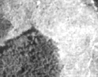
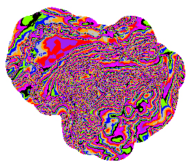
Each of these raster data sets have essentially the same tessellated structure. Here are few graphical examples of raster data:

A simple scanned photographic image.

Some 8-bit digital orthophotos.
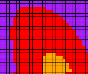
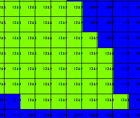
Three different views of a classified elevation grid, showing cell outlines and elevation values.
As you can see, when the images are blown up in size, the pixels become visible.
USGS DEMs (Digital Elevation Models) are ASCII files which contain georeferencing information as well as point data for elevations on the surface of the earth. Here are the first 4 lines in the Eatonville, WA 7.5' 30 m DEM:
EATONVILLE, WA 464512215 80000 HAP-81 78-73 08/06/81 BC2 30MX30M INTERVA
EATONVILLE, WA 464512215 FS 1 1 1 10 0.000000000000000D+00
0.000000000000000D+00 0.000000000000000D+00 0.000000000000000D+00
0.000000000000000D+00 0.000000000000000D+00 0.000000000000000D+00
0.000000000000000D+00 0.000000000000000D+00 0.000000000000000D+00
0.000000000000000D+00 0.000000000000000D+00 0.000000000000000D+00
0.000000000000000D+00 0.000000000000000D+00 2 2 4 0.547738572300000D+06
0.517735436400000D+07 0.547628092800000D+06 0.519124459100000D+07
0.557153679500000D+06 0.519132801700000D+07 0.557286257000000D+06
0.517743781300000D+07 0.133000000000000D+03 0.987000000000000D+03
0.000000000000000D+00 10.300000E+020.300000E+020.100000E+01 1 322

1 1 92 1 0.547650000000000D+06 0.518850000000000D+07 0.0
0.170000000000000D+03 0.271000000000000D+03 214 214 215 215 221 227 233
240 246 252 257 261 266 264 262 260 262 263 265 266 266 267 268 269 271
270 269 268 268 268 268 267 265 264 263 262 261 261 261 261 260 259 258
258 258 258 256 254 251 245 239 233 229 225 221 216 212 208 204 200 196
194 192 190 190 190 191 190 190 189 189 188 188 188 188 189 188 187 187
187 186 186 184 183 181 180 179 177 175 173 172 170

1 2 218 1 0.547680000000000D+06 0.518472000000000D+07 0.0
0.133000000000000D+03 0.425000000000000D+03 393 396 400 403 408 414 419
421 423 425 423 422 420 412 403 395 391 386 382 373 365 357 347 338 329
324 318 313 312 312 311 308 305 302 301 300 299 297 295 293 289 285 281
279 277 275 270 265 260 253 247 241 233 226 218 216 213 211 209 207 205
205 205 204 202 200 197 197 197 197 197 197 198 199 200 201 206 211 216
218 219 221 216 211 207 186 166 145 142 138 135 135 135 135 135 135 135
134 134 133 134 135 136 135 135 134 148 163 177 185 192 200 202 203 205
206 208 209 210 212 213 213 213 213 213 214 214 214 214 215 219 224 229
235 241 248 253 258 263 262 261 260 261 263 265 266

266 267 268 269 270 269 268 267 267 267 267 265 264 263 262 261 259 260
260 261 259 257 255 255 255 254 252 250 248 243 238 233 228 224 220 216
212 207 204 200 197 195 193 192 191 191 191 190 190 189 189 188 188 188
188 188 188 187 187 186 186 186 184 183 182 180 179 177 176 174 172 171
The first line lists the file name, data input type (HAP = High Altitude Photography), cell size (30MX30M). The subsequent lines list elevations for the lattice mesh points (cell centers).
USGS DEMs are imported into ARC/INFO using the DEMLATTICE command:
Arc: demlattice q1822.dem eaton
 Dem file q1822.dem does not exist.
Arc: demlattice q1822 eaton
Loading header information...
Datum and Spheroid are missing.
Deducing from DEM projection...
Datum - NAD27, Spheroid - Clarke 1866.
DEM extent [547628.093, 5177354.364, 557286.257, 5191328.017]...
DEM surface range [133.000, 987.000]...
Sample distance in x and y [30.000, 30.000]...
Reading in lattice...100%
Rotating lattice...
Percentage : 100%
Output lattice is 322 points in x, and 466 points in y.
Describing Spatial Data in ARC/INFO
To list spatial data sets that exist in a workspace, use these commands to list, respectively, coverages, grids, TINs, and images.
Arc: lc
Arc: lg
Arc: lt
Arc: listimages
Before you do anything with spatial data sets in ARC/INFO, you should DESCRIBE the coverage, grid, or TIN you are interested in:
Arc: describe ponet
                 Description of SINGLE precision coverage ponet
                                FEATURE CLASSES
                                    Number of  Attribute     Spatial
Feature Class          Subclass     Features   data (bytes)  Index?   Topology?
-------------          --------     ---------  ------------  -------  ---------
ARCS                                      429        32
POLYGONS                                  144        62               Yes
NODES                                     412
ANNOTATIONS             (blank)            25
                               SECONDARY FEATURES
Tics                                        4
Arc Segments                             8855
Polygon Labels                            143
                                   TOLERANCES
Fuzzy   =                47.466 V          Dangle  =                 0.000 N
                               COVERAGE BOUNDARY
Xmin =               342364.719            Xmax =               736453.000
Ymin =              4982733.000            Ymax =              5542725.000
                                     STATUS
The coverage has not been Edited since the last BUILD or CLEAN.
                          COORDINATE SYSTEM DESCRIPTION
Projection                  UTM
Zone                         10
Units                    METERS             Spheroid             CLARKE1866
Parameters:
The description will tell you how many of each spatial feature types exist in the coverage (here we have arcs with an AAT, polygons with a PAT, nodes, annotations, and tics). Annotations are text features marking geographic locations, such as road or stream names. The description includes the actual number of arc segments and polygon labels (polygon labels should number 1 less than the number of polygons). Coverage boundary and edit status is also listed, and finally, the coordinate system is detailed. In order for any data sets to match each other spatially, they must share a common coordinate system.
When grids are described, the output is similar:
Arc: describe eaton
                           Description of Grid eaton
Cell Size =              30.000         Data Type:            Floating Point
Number of Rows    =         466
Number of Columns =         322
           BOUNDARY                                STATISTICS
Xmin =               547635.000         Minimum Value =              133.000
Xmax =               557295.000         Maximum Value =              987.000
Ymin =              5177355.000         Mean          =              384.782
Ymax =              5191335.000         Standard Deviation =         134.236
                          COORDINATE SYSTEM DESCRIPTION
Projection                  UTM
Zone                         10
Datum                     NAD27
Zunits                   METERS
Units                    METERS             Spheroid             CLARKE1866
Parameters:
The grid description lists the cell size, the number of rows and columns, data type (floating point or integer), boundary, basic cell value statistics, and coordinate system information.
Basic display of spatial data is done using the ArcPlot module. ArcPlot has a range of functions, from performing quick query and display, to creating cartographic-quality maps. To start ArcPlot, enter "AP" at the Arc: prompt. Following are a few basic commands to get you started.
Setting up display
Setting spatial extent
Displaying spatial data
Setting up display:
If a graphical display window does not automatically appear, enter "&stat
9999". This loads a station file, which sets input and output devices,
most importantly, the display window.
Setting spatial extent:
ArcPlot displays all spatial data in reference to absolute coordinates.
When the display window is invoked, its "map extent" is undefined.
To set a different spatial extent of display, it is necessary to use the
MAPEXTENT command:
Arc: ap
Copyright (C) 1982-1997 Environmental Systems Research Institute, Inc.
All rights reserved.
ARCPLOT Version 7.1.2  (Wed Aug 13 07:45:00 PDT 1997)
Arcplot: &stat 9999
Arcplot: show mape
WARNING the Map extent is not defined
   .9990000000000E+36,   .9990000000000E+36,
   -.9990000000000E+36,  -.9990000000000E+36
Arcplot: mape eaton
Arcplot: show mape
	546935.9999895,5176655.999989,557994.0000104,5192034.00001
Note how the map extent is initially set to an outrageously large area, and after setting to the boundary for a specific data set, the map extent is within reasonable limits.
Displaying spatial data
Once your map extent is set to display the area you want, you are ready
to begin displaying data.
POINTS (or LABELS for a polygon cover):
To draw points or labels for a coverage, use the command(s)
Arcplot: points <cover>
Arcplot: labels <cover>
To draw points or labels for a coverage using a specific symbol, use the command(s)
Arcplot: pointmarkers <cover> {symbol | item}
Arcplot: labelmarkers <cover> {symbol | item}
To display an attribute for a point or polygon coverage, use the command(s)
Arcplot: poinntext <cover> <item>
Arcplot: labeltext <cover> <item>
ARCS:
To draw arcs for a coverage, use the command
Arcplot: arcs <cover>
To draw arcs for a coverage using a specific symbol, use the command
Arcplot: arclines <cover> {symbol | item}
To display an attribute for an arc coverage, use the command
Arcplot: arctext <cover> <item>
POLYGONS:
To draw polygon outlines for a coverage, use the command
Arcplot: polys <cover>
To draw polygon outlines for a coverage using a specific symbol, use the command
Arcplot: polygonlines <cover> {symbol}
To draw filled polygons for a coverage using a specific symbol, use the command
Arcplot: polygonshades <cover> {symbol | item}
To display an attribute for a polygon coverage, use the command
Arcplot: polygontext <cover> <item>
Note that these commands apply to selected features only. If you have active selections (see RESELECT, ASELECT, NSELECT), only selected features will be displayed.
You can clear the display using the CLEAR command
Queries on vector data generally take the form of:
Where are features with a given attribute?
or
What feature is at a given location?
To find features with given attributes, select the feature(s) of interest and display them. Most of the ArcPlot display commands respect selected sets, that is, if a certain set of polygons in a coverage is selected, then the polygonshades, polygons, and polygonlines commands will display only those selected polygons.
The basic commands you should be aware of for query and display are:
POINTS <cover> {NOIDS | IDS | IDSONLY}

LABELS <cover> {IDS | IDSONLY | NOIDS}

ARCS <cover> {NOIDS | IDS | IDSONLY}

ARCLINES <cover> {item | symbol} {lookup_table}

ARCTEXT <cover> <item> {lookup_table}
               {POINT1 | POINT2 | LINE} {offset}
               {LL | LC | LR | CL | CC | CR | UL | UC | UR | BLANK} {NOFLIP}

POLYGONS <cover>

POLYGONLINES <cover> {item | symbol} {lookup_table} {NOISLANDS}

POLYGONSHADES <cover> <item | symbol> {lookup_table}
                     {angle_item | angle}
Here are a few examples:
Arcplot: reselect str2 arc str2dnrty = 1
Arcplot: arcs str2
will display only streams which have a DNR type of 1
Arcplot: reselect tty4 poly age_1998 lt 20 and age_1998 gt 0
Arcplot: polygonlines tty4 2
will display polygon outlines (in symbol line symbol 2) for stands within the ages of 0 and 20.
To find features based on their location, use the IDENTIFY command:
Arcplot: IDENTIFY <cover> <feature_class> <* | xy> {item...item}
Arcplot: IDENTIFY <cover> EVENT <route_system> <* | xy>
                <<event_source> {item...item}...
                AND <event_source> {item...item}>
Arcplot: IDENTIFY <FIRST | ALL>
The first 2 usage statements give the option for interactive location ("*") or coordinate location ("xy"). The first 2 statements also give options for which attribute table items to list. If no attribute items are given, then values for all items will be listed. Note that the coverage name and feature type are necessary arguments.
Here are a few examples:
Arcplot: identify tty4 poly * est_year unit_name asp_meanwill display only the establishment year, management unit name, and mean aspect for the stand which is clicked.
Arcplot: iden rds2 arc 1197768 555485will display all arc attributes for the road which passes near 1197768 555485.
If you attempt an identify and receive the message:
No feature located.
one of several things has happened:
Although attributes are alluded to here, attribute values are the topic of the next lesson.