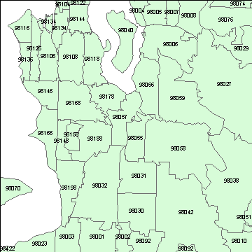
Figure 1: ESRI ZIP code boundaries from the ESRI Maps and Data DVD for 2007:
This document describes very briefly the differences between ZIP code "areas" and ZCTAs.
What are ZIP codes?
ZIP (acronym for Zone Improvement Plan) codes were implemented in 1963 as a method to improve mail delivery service. ZIP code areas are technically not areas in the geometric sense, they are essentially lists of addresses that are used to make delivery of mail more efficient. ZIP code polygons can be constructed by grouping addresses and then circumscribing polygons around addresses with the same ZIP code. This is what commercial vendors of ZIP code boundaries do.
What are ZCTAs?
ZCTAs (acronym for ZIP Code Tabulation Areas). A good description of ZCTAs can be found at the US Census ZCTA FAQ. Specifically, from the FAQ:
Is there an equivalency or comparability data product that shows the relationship between Census 2000 ZCTAs™ (ZIP Code Tabulation Areas) and USPS 2000 ZIP Codes?
The Census Bureau is not planning to produce a 2000 ZIP Code to 2000 ZCTA relationship file. We created the ZCTAs specifically to address the inadequacies of ZIP Codes for census data tabulation.
For those who may want to do this, the TIGER/Line® files will continue to show address ranges with mailing ZIP Codes. These files can be processed using a GIS to compare the ZCTA code for a block to the mailing ZIP Code associated with the address ranges on each block side. Such a comparison can provide a general idea of how the two relate.
The relationship between ZIP Code and ZCTA can be determined fully only by comparing individual block-geocoded addresses to the ZCTAs. This process is quite involved. Some examples of why the process can become quite involved are as follows: ZCTAs follow census block boundaries. In contrast, USPS ZIP Codes serve addresses with no correlation to census block boundaries; therefore, the area covered by a ZCTA may include mailing addresses associated with ZIP Codes that are not the same as the ZCTA.
A ZCTA may include a mailing address with a unique or PO Box ZIP Code that is ineligible to become a ZCTA. Addresses with PO Box ZIP Codes generally cluster around a post office, but they may be widely scattered across several ZCTAs. Consequently, the relationships that exist between ZCTAs and ZIP Codes can become quite complicated, so that within the boundaries of a single ZCTA there may exist several ZIP Codes; likewise, within the boundaries of a single ZIP Code, there may exist more than one ZCTA.
Some addresses included in the census and used to define ZCTAs (typically in rural areas) have incomplete or, in some cases, no mailing ZIP Code, thus making it difficult to determine the full extent of the relationships between ZCTAs and ZIP Codes.
How different are ZIP code areas and ZCTAs?
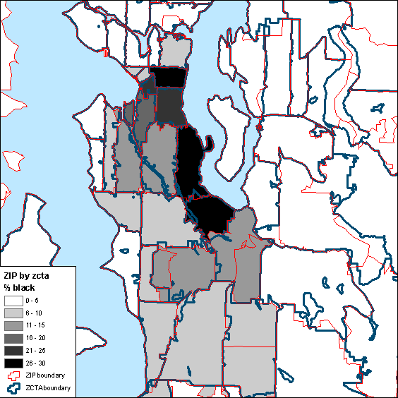
In some cases, they are very similar. In other cases not as similar as we would like. The following set of 3 images demonstrates this. Draw your attention to ZIP 98166 (Figure 1) & ZCTA 98116 (Figure 2) at the northwest corner of the map. The boundaries are nearly identical (a best case scenario). Now draw your attention to ZIP 98055 and 98057 (Figure 1, in the center of the map). Note that ZCTA 98057 does not exist.
Figure 1: ESRI ZIP code boundaries from the ESRI Maps and Data DVD for 2007:
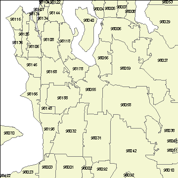
Figure 2: ZCTAs from US Census TIGER/Line files (2000)
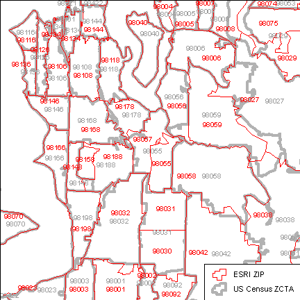
These differences can be visualized more clearly by displaying both sets of data on one map (Figure 3). Specifically, look at ZCTAs 98055 (center), 98188 (just west of 98188), and 98031 (south-central). Some ZCTAs appear to be split rather cleanly into two ZIPs (e.g., ZCTA 98031) and others are less well behaved (e.g., ZIP 98027).
Figure 3: ZIP and ZCTA boundaries
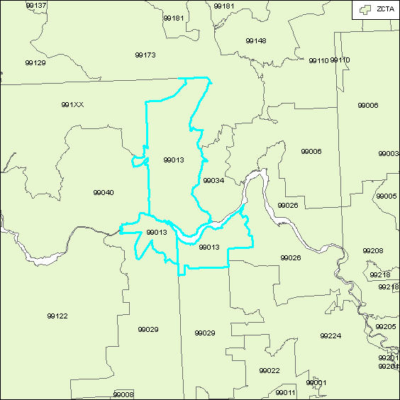
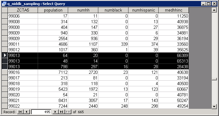
Furhtermore, many ZCTAs in the US Census data are represented by more than one polygon (e.g., where they span county boundaries), as shown in Figure 4.
Figure 4a: Multiple polygons for ZCTA 99013
Figure 4b: Multiple database records for ZCTA 99013
Why is this a problem?
We have detailed demographic data from the US Census for ZCTAs. We do not have demographic data for ZIP code areas. It is possible to use area-weighted methods to apportion statistics from ZCTAs to ZIP code areas. Suppose a sampling scheme were developed for randomly selecting households based on Census variables from ZCTAs (e.g., poverty status or race). A number of households will be specified for random selection from a given ZCTA or group of ZCTAs. Suppose that group includes ZCTA 98055. That list of ZCTAs is passed to a company that specializes in operationalizing surveys. They pass the list of ZCTA numbers to their telephone exchange number vendor. The telephone exchange provider selects exchanges that are in ZIP (not ZCTA) 98055. The problem is that the neither the survey contractor nor the telephone number vendor has been told to also select telephone numbers from ZIP 98057 (which does not exist as a ZCTA). Thus, there will be "holes" in the list of selected telephone numbers.
Using GIS to overlay the data sets and compute area proportions can be used to assign ZCTA statistics to the ZIP code areas. For example, ZCTA 98031 is about 50% ZIP 98031 and 50% 98030. Also consider ZIP 98056, which completely contains ZCTA 98056 but also part of ZCTA 98059. Also, ZIP 98027 is split by ZCTAs 98059 and 98027.
How to deal with this
Imagine if you had a jigsaw puzzle with pieces in the shape of ZCTAs made of cookie dough. Each puzzle piece is a different thickness (proportional to the value of a demographic variable). Now get a set of cookie cutters that are the shape of ZIP code areas and cut the puzzle with the new cookie cutters. Push the dough down into each new cookie cutter so it is completely level within each individual cutter. These heights are the new recalculated values. Do this for various puzzles where each puzzle starts with pieces with different thicknesses (these correspond to each census demographic variable). Operationally:
| SELECT SF3GEO.ZCTA5, Sum(SF30001.P001001)
AS population, Sum(SF30001.P010001) AS numhh, |
| # handle proportions of zip & zctas # read the data in from GDB #ZCTA census data # merge # proportion of ZCTA in this ZIP # multiply the proportion of ZCTA in this ZIP by the counts in the ZCTA # now sum each proportionalized variable per ZIP # combine variables into a data frame # calculate percentages # join the ZCTA values for comparison # a plot of recalculated (ZIP) vs original (ZCTA) values #write the values out colnames(zip.demog1) <- unfix.colnames(zip.demog1)
|
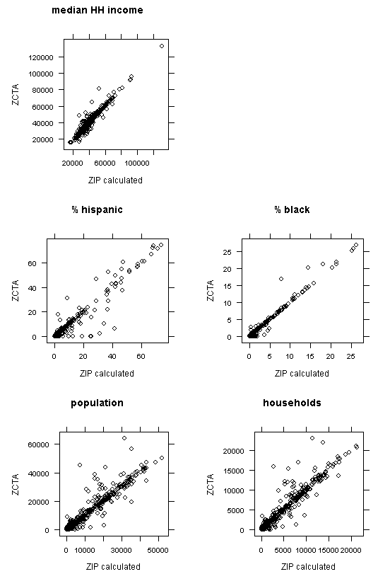
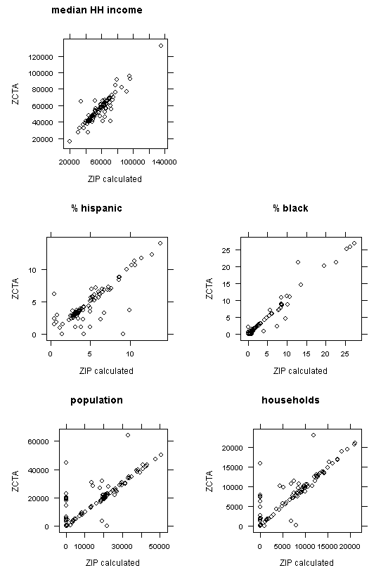
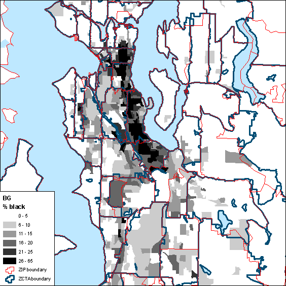
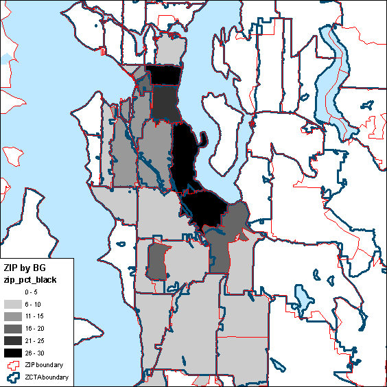
Potentially better results can be obtained by aggregating from census block groups to ZIP code areas, because the original block group data contain more spatial variation than do ZCTA data. Figure 7 displays percent of residents that are black at the block group level (raw data; the smallest available spatial unit with these variables). Figure 8 shows a scatter plot of ZCTA data and re-aggregated block group data. How to do this is left as an exercise for the reader.
Figure 7: Percent of residents that are black by census block group (upper), block group data aggregated to ZIP code area (middle), and ZCTA data aggregated to ZIP code area (lower)
Figure 8: Scatter plots of demographic variables comparing original ZCTA and ZIP code area data re-aggregated from block groups (King County only)